Casualty
Accident Casualty
In this section, we will focus on the casualty of car accidents. More specifically, we will visualize the distribution of killed or injured people among different boroughs.
People Injured by Borough
injured_borough_box =
  accidents1 %>%
  filter(!is.na(borough)) %>%
  plot_ly(x = ~number_of_persons_injured, color = ~borough, type = "box", colors = "viridis") %>%
  layout(title = "<b>Number of Injuries by Borough</b>",
         xaxis = list(title = "Number of People Injured"))
injured_borough_box
In each crash accident, Manhattan has the least serious injuries, and the other boroughs have similar injury amounts. However, Brooklyn has the largest number of injuries which is 15. The number of deaths in 5 boroughs are similar and not large. The median number of fatalities per crash is 0. However, Brooklyn also has the largest number of fatalities which is 3. Based on the information above, it can be concluded that Brooklyn has the most serious car accident fatality.
People Killed by Borough
killed_borough_box =
  accidents1 %>%
  filter(!is.na(borough)) %>%
  plot_ly(x = ~number_of_persons_killed, color = ~borough, type = "box", colors = "viridis") %>%
  layout(title = "<b>Number of People Killed by Borough</b>",
         xaxis = list(title = "Number of People Killed"))
killed_borough_box
In each crash accident, Manhattan has the least serious injuries, and the other boroughs have similar injury amounts. However, Brooklyn has the largest number of injuries which is 15. The number of deaths in 5 boroughs are similar and not large. The median number of fatalities per crash is 0. However, Brooklyn also has the largest number of fatalities which is 3. Based on the information above, it can be concluded that Brooklyn has the most serious car accident fatality.
People Injured and Killed by Borough
injured_killed_bar =
accidents1 %>%
  dplyr::select(borough, number_of_persons_injured, number_of_persons_killed) %>%
  group_by(borough) %>%
  mutate(injuries_total = sum(number_of_persons_injured),
            killed_total = sum(number_of_persons_killed)) %>%
  dplyr::select(borough, injuries_total, killed_total) %>%
  unique() %>%
  filter(!is.na(borough)) %>%
  pivot_longer(
    injuries_total:killed_total,
    names_to = "types_of_casualties",
    values_to = "number_of_casualties")

injured_killed_bar_plot =
  injured_killed_bar %>%
  mutate(borough = as.factor(borough),
         borough = fct_relevel(borough, "NA", "Brooklyn", "Queens", "Bronx", "Manhattan", "Staten island")) %>%
ggplot(aes(x = borough, y = number_of_casualties, fill = types_of_casualties)) +
  geom_bar(stat = "identity",
           position = "dodge",
           width = 0.8) +
  geom_text(aes(label = number_of_casualties),
            size = 4,
            position = position_dodge(width = 0.8),
            vjust = -0.3) +
  labs(
    title = "Frequency of Casualties in Boroughs",
    x = "Borough",
    y = "Number of Casualties in Each Borough",
    fill = "Types") +
  theme_bw(base_size = 12) +
  theme(axis.text = element_text(colour = 'black'),
        plot.title = element_text(hjust = 0.5)) +
   ylim(0, 6500)
injured_killed_bar_plot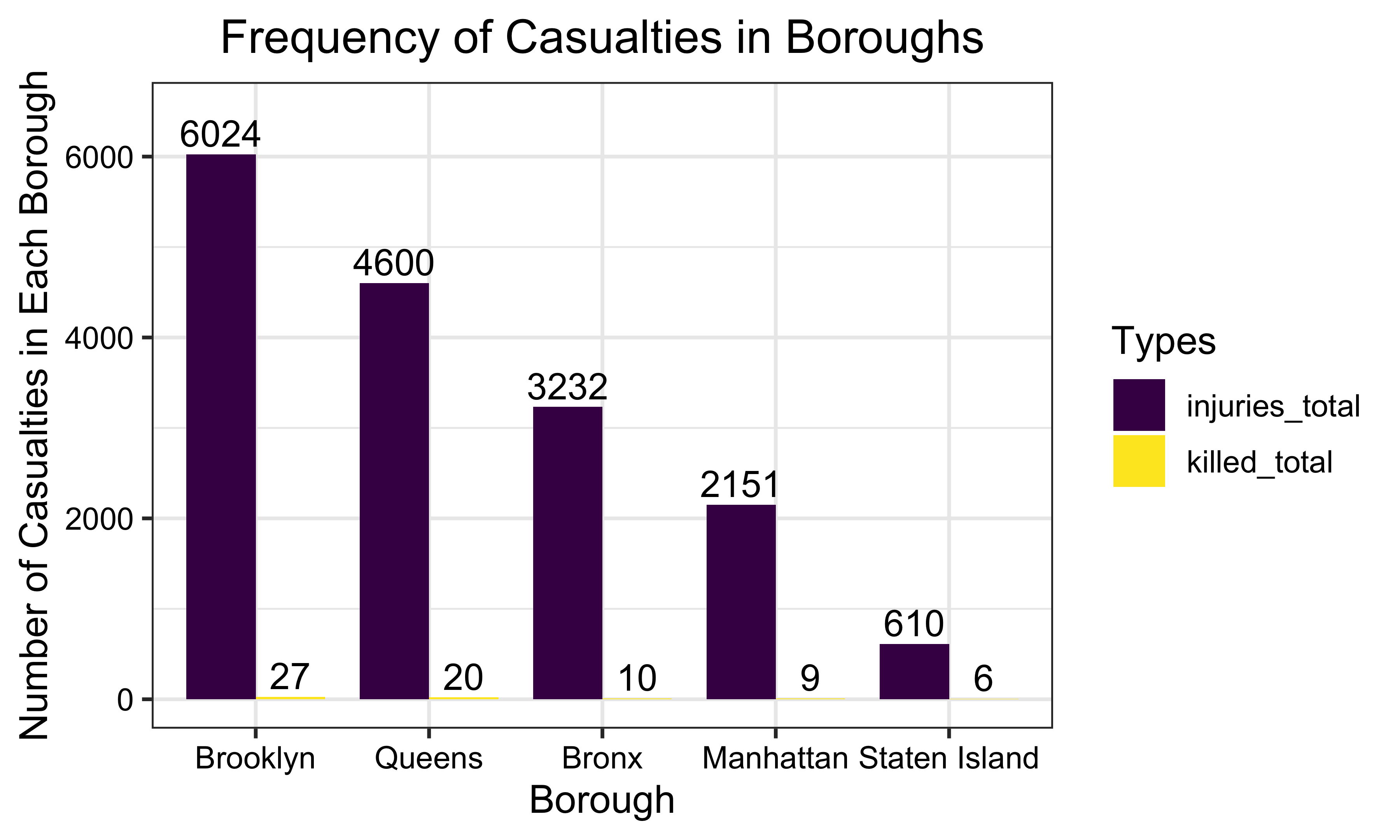
From January 2020 to August 2020, Brooklyn had the largest total number of injuries and fatalities. Conversely, Staten Island had the lowest total number of injuries and fatalities in car accidents.
The following two plots show the number of injured and killed people separately.
Total Number of People Injured by Borough
casualties_table =
accidents1 %>%
  group_by(borough) %>%
  summarize(injuries_total = sum(number_of_persons_injured),
  killed_total = sum(number_of_persons_killed)) %>%
  filter(!is.na(borough))

injuries_borough_plot =
casualties_table %>%
  mutate(borough = forcats::fct_reorder(borough, injuries_total, .desc = TRUE)) %>%
  ggplot(aes(x = borough, y = injuries_total, fill = borough)) +
  geom_bar(stat = "identity",
           width = 0.8) +
  geom_text(aes(label = injuries_total),
            size = 4,
            position = position_dodge(width = 0.8),
            vjust = -0.3) +
  labs(
    title = "Frequency of People Injured in Boroughs",
    x = "Borough",
    y = "Number of People Injured in Each Borough") +
  theme_bw(base_size = 12) +
  theme(axis.text = element_text(colour = 'black'),
        plot.title = element_text(hjust = 0.5)) +
  ylim(0, 6500)
injuries_borough_plot
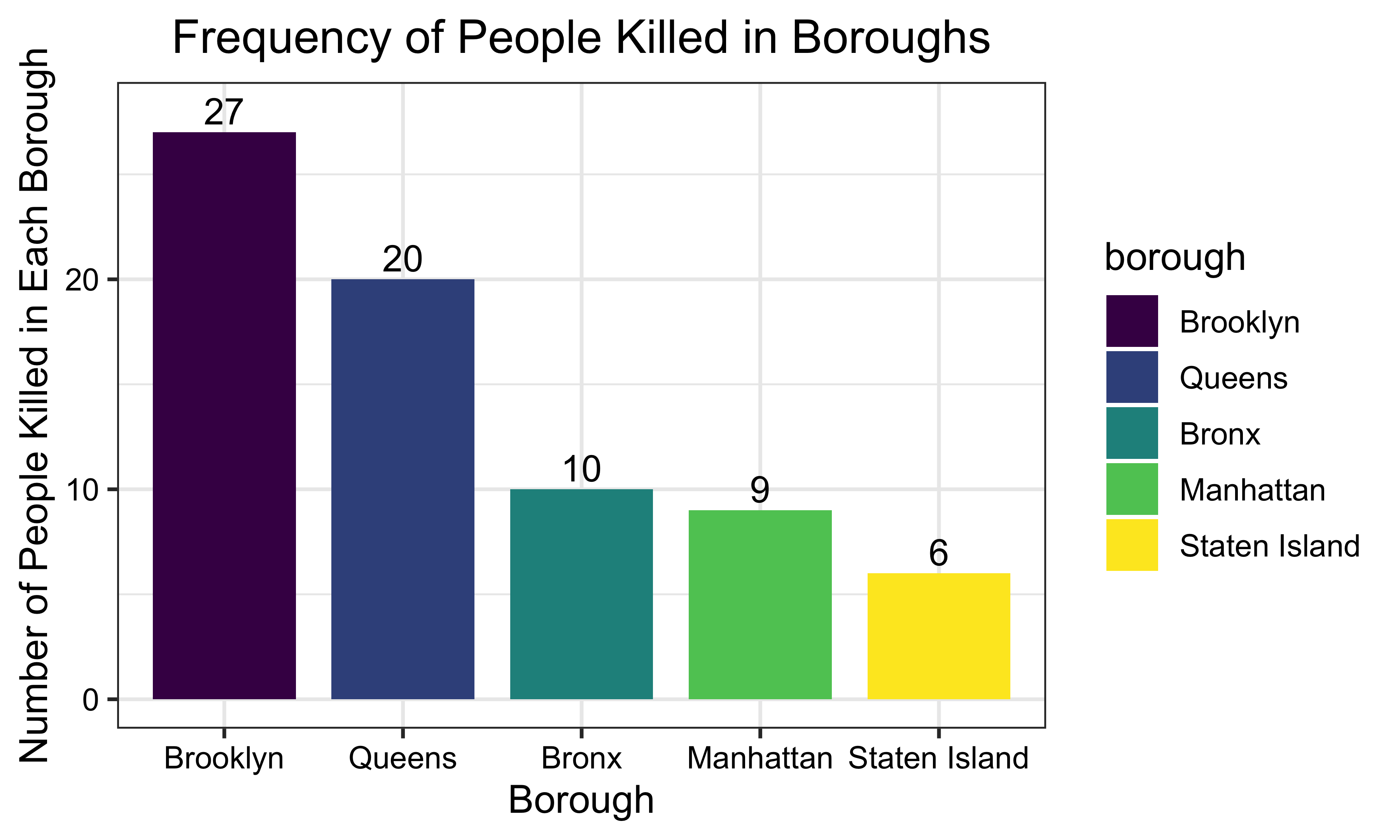
Total Number of People Killed by Borough
killed_borough_plot =
casualties_table %>%
  mutate(borough = forcats::fct_reorder(borough, killed_total, .desc = TRUE)) %>%
  ggplot(aes(x = borough, y = killed_total, fill = borough)) +
  geom_bar(stat = "identity",
           width = 0.8) +
  geom_text(aes(label = killed_total),
            size = 4,
            position = position_dodge(width = 0.8),
            vjust = -0.3) +
  labs(
    title = "Frequency of People Killed in Boroughs",
    x = "Borough",
    y = "Number of People Killed in Each Borough") +
  theme_bw(base_size = 12) +
  theme(axis.text = element_text(colour = 'black'),
        plot.title = element_text(hjust = 0.5)) +
  ylim(0, 28)
killed_borough_plot